This page is maintained by the software tutors. For errors and/or amendments please contact the current tutor supporting the program.
Introduction
Stata is among the most popular software packages for performing econometric analyses. It features a large set of econometric techniques and efficient data handling procedures. Users without any background in command-oriented software may find the first steps difficult, but once the basic principles are understood, the software allows for easy access to a wide set of different estimators.
Stata can be used in three different ways. In the interactive mode you directly type the commands in the command window. If you're unfamiliar with the syntax of a particular command you can execute it via menus as in any other Windows software. Newcomers may find this option particularly attractive. As you become more familiar with Stata you may want to work with do-files. They allow for fast execution of command sequences such that you work more efficiently. If you use the menus Stata generates code that you then can copy into the do-file.
Main types of variables: .dta data files; .do command files; .ado programs or commands; .hlp help files; and .gph graphs.
Load, open and save Stata format files (.dta):
First: set the memory (in the versions below 12)
set mem 200m
Second: load the file
use "U:\Working\data\2011.dta", clear
(clear: delete all the data which the memory is using)
Third: work with the data base and save it:
save "U:\Working\data\2011.dta", replace
If you use the same directory you can fix it:
cd "U:\Working\data\"
and then
use "2011.dta", clear
and
save "2011.dta", replace
(saveold "2011.dta", replace)
in the version12 in order to use the database in older versions.
If you want to use some variables (month, gender, labor, wages) you can:
use year gender labor using "U:\Working\data\2011.dta"
Data Description
To see the names of variables, type of variable (numeric or string):
describe (des)
To see the basic statistics (number of observations, mean, standard deviation, min, and max ) of each variable:
summarize (sum)
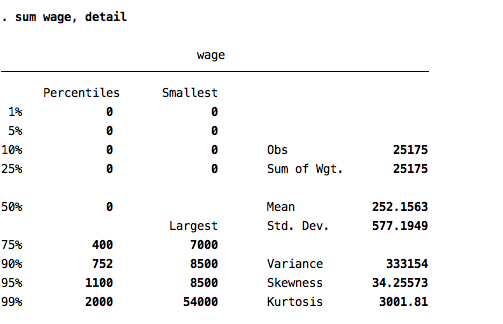
If you want the percentiles, the skewness and the kurtosis:
summarize, detail (sum, detail)
If you want apply these commands for a set the variables you write the name of the variable after the command
sum labor, detail
If you want to see the frequency you can tabulate the variables (one way):
tabulate (tab) labor
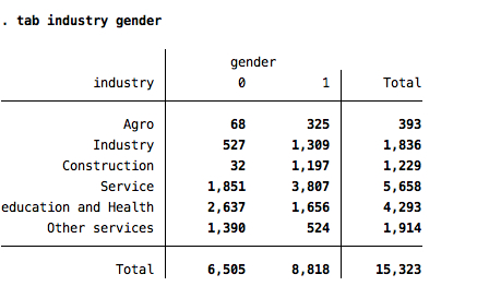
Two ways:
tabulate (tab) gender labor
Considering the missing observations
tab gender labor, missing (m)
Restricting for some group (e.g. only in June)
tab gender labor if month==6,m
Basic Commands
If you want generate a new variable
Generate the logarithm of the wages
generate (gen) lwage=log(wage)
Generate a dummy variable (0 or 1) if the individual is unemploy (e.g in the labor variable it is the number 2)
gen unemploy=0
replace unemploy=1 if labor==2
or also to generate a dummy variable for each labor condition (you can generate with the name labor1, labor2, labor3…)
tab labor, g(labor)
another example generating a new variable:
gen quarter=.
replace quarter=1 if month>=1 | month<4
replace quarter=2 if month>=4 | month<7
replace quarter=3 if month>=6 | month<10
replace quarter=4 if month>=9 | month<=12
Generating a variable indicating some order for example by income:
sort income
gen id=_n
Other examples
gen abs_diff=abs(wage-taxes)
gen sqage=age^2
gen ones=1
Putting a new name:
rename sqage age2
Recoding:
recode gender 2=0
Using recode to create a new variable:
recode month (1/3=1) (4/6=2)(7/9=3)(10/12=4), gen(quarter)
Keeping and dropping cases:
drop if wage==0
keep if age>17
egen creates newvar of the optionally specified storage type equal to function(arguments). Here function() is a function specifically written for egen, as documented below or as written by users. Only egen functions may be used with egen, and conversely, only egen may be used to run egen functions.
egen sumwage=sum(wage)
egen meanwage=mean (wage), by (gender)
Other functions:
min Minimum value
max Maximum value
mean mean
median median
pctile percentile
sd standard deviation
Basic loop, generate a variable wage for each quarter:
foreach quarter in 1-4 {
gen wage`num'= wage if quarter==`num'
}
Another way:
forval x = 1/4 {
gen wage`x’=wage if quarter==`x’
}
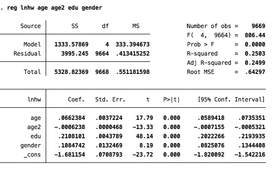
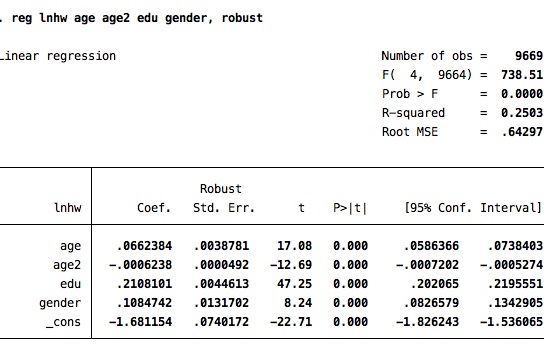
Simpler linear regression:
reg lwage education age age2 gender
reg lwage education age age2 gender, robust (control by heterocedasticity)
reg lwage education age age2 gender, noconstant (without constant)
reg lwage education age age2 gender [aw=weight] (weighting)
postestimation:
predict lwage_est
( xb linear prediction; the default)
predict res, r
There are more options in help regress_postestimation
Logistic regression:
logit success education age age2 gender
logit success education age age2 gender, robust (control by heterocedasticity)
logit success education age age2 gender, noconstant (without constant)
logit success education age age2 gender [aw=weight] (weighting)
logit success education age age2 gender, or (odds ratios)
postestimation:
predict yhat, pr
(probability of positive outcome, the default)
predict yhat, xb
( xb linear prediction)
predict res, r
(residuals)
There are more options in help logit_postestimation
Export regressions to Latex:
eststo: reg lwage education age age2 gender
eststo: reg lwage education age age2 if gender==1
eststo: reg lwage education age age2 if gender==0
estout, cells(b(star fmt(a3)) se(fmt(2) par)) starlevels(* 0.10 ** 0.05 *** 0.01)stats(r2 N, fmt(3 0)) style(tex) varlabels(_cons _cons)
Graphics
Stata has a powerful and extensive graphics' package. Here I will present some examples but there are many examples and personalized tool that you can see with the command help:
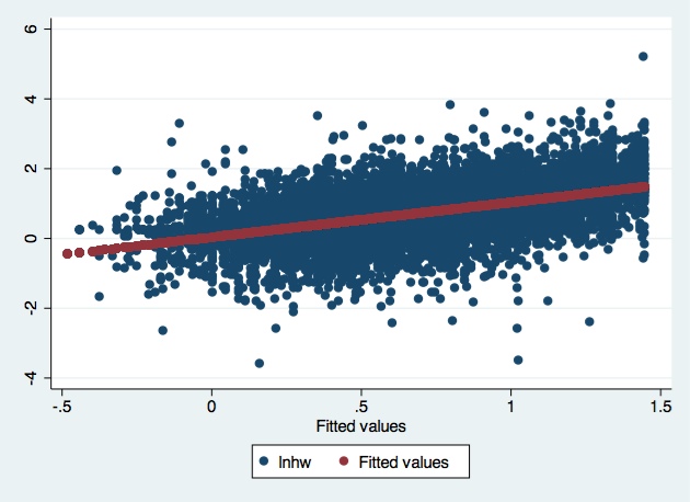
Dipersion graph
twoway (scatter lwage education)
(scatter lwage education)
Dispersion graph by gender group
twoway (scatter lwage education), by(gender)
(scatter lwage education), by(gender)
Dispersion graph with linear approximation
twoway (scatter lwage education) ///
(lfit lwage education) , ///
ytitle(Wages (Ln)) xtilte(Education)
Histograms
hist education, freq
Bar-Charts
graph bar education, by(gender)
graph bar gender, by(education)
Page last updated on 17 August 2017